The Platonic Representation Hypothesis in a Small World: Tic-Tac-Toe

Luc Pommeret

Introduction

LLMs are models whose performance on human language is no longer in question. Based on the transformer architecture, their extraordinary capabilities sometimes seem to elude us, to the point where we don't always understand how the model infers what it infers.

One hypothesis in particular has caught our attention because it seems to synthesize many scattered observations we've made in the field of interpretability (or explainability). This is the PRH, or Platonic Representation Hypothesis, which postulates that transformer models forge a model of world representation during training, resulting from the search for simplicity that a learning neural network naturally seeks.

The most surprising consequence of their hypothesis is that models trained on different types of data (images, text, sounds, etc.) will converge towards the same representation in their latent space. Our goal here will be to study in depth a simple, very simple case, that of Tic-Tac-Toe. In this game, where all possible games can be generated in a few minutes by a modern computer, the world is very simple, and does not require immense computing power, another advantage we can take advantage of.

Here we will study the representations of two transformers: one is trained on images of the game, and the other on sequences of moves in text form.

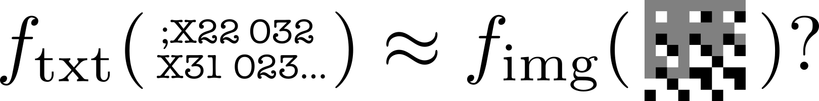
The main hypothesis we want to test is essentially whether the two representations of the same Tic-Tac-Toe game converge.

To prepare the ground and explore other aspects of interpreting the transformer architecture, we will perform tests using other techniques, starting with probing.

How to represent a Tic-Tac-Toe game?

Tic-Tac-Toe, like chess or checkers, is a board game. But unlike the latter two, it is extremely simple, which allows for completeness of analysis (we generate all possible games and analyze our transformer with all these games).

A very simple, even childish way to represent a Tic-Tac-Toe game is to note it in the form of a drawing, side by side, showing the state of the board at each move. This is the format we chose for the images, which therefore have a size of 9x9.

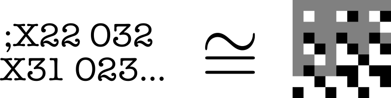
To note Tic-Tac-Toe games textually, we chose to note the moves one after the other, like the PGN format in chess, which gives a history of the game.

Given the format of the Tic-Tac-Toe game, the number of moves cannot exceed 9, which is very convenient for tokenization, the first step in learning.

Here are the respective tokenizations of images and texts (found in the meta.pkl files):

{
"vocab_size": 4,
"itos": {"0": "b", "1": "n", "2": "g", "3": ";"},
"stoi": {"b": 0, "n": 1, "g": 2, ";": 3}
}
            

{
"vocab_size": 10,
"itos": {"0": ";", "1": " ", "2": "0", "3": "1", "4": "2", "5": "3", "6": "X", "7": "O", "8": "/", "9": "-"},
"stoi": {";": 0, " ": 1, "0": 2, "1": 3, "2": 4, "3": 5, "X": 6, "O": 7, "/": 8, "-": 9}
}
            

The stoi and itos are not Greek, but a data format that allows converting strings to integers, that is, string to integer or more simply stoi, with itos being the reciprocal operation.

The tokenization of images is based on the pixel, which will be white, value 0 (represented by 'b'), if the cell is saturated by an X, black, value 1 (represented by 'n'), if the cell is saturated by an O, and gray, value 2 (represented by 'g') if the cell is empty. The image is traversed naturally, line by line to form a line in str (string) format.

In both cases, ";" is the start token, which marks the beginning of the sequence for both images and texts.

Probing

Probing is a technique for detecting the presence of properties in a neural network. It's a technique that has been extensively used since 2018 and Manning et al.'s article applying it to the detection of syntactic trees in a transformer trained on a corpus of tagged texts.

Here, we want to use probing to detect the presence or absence of a representation of the Tic-Tac-Toe board, layer by layer in the transformer. The idea is to train a linear classifier cell by cell and layer by layer to detect the state of a cell (X, O, or empty). The technique used here is a generalization of the original SVM, called OneVsRest.

What is a linear SVM?

The linear SVM (Support Vector Machine) is a supervised learning technique used for classification. In the binary case, the objective is to find a hyperplane that best separates the two classes of data. In the linear case that concerns us, it is therefore a matter of finding the hyperplane that best explains the separation of data in the neural network.

Let a training data set \(\{(x_i, y_i)\}_{i=1}^n\), where \(x_i \in \mathbb{R}^d\) are the feature vectors and \(y_i \in \{-1, +1\}\) are the class labels.

The separating hyperplane is defined by the equation:

\[w^T x + b = 0\]

where \(w \in \mathbb{R}^d\) is the normal vector to the hyperplane and \(b \in \mathbb{R}\) is the bias.

Optimization Problem

The SVM seeks to maximize the margin between the hyperplane and the closest points of each class. This translates into the following optimization problem:

\[ \begin{aligned} \min_{w,b} &\quad \frac{1}{2} \|w\|^2 \\ \text{s.t.} &\quad y_i(w^T x_i + b) \geq 1, \quad i = 1, \ldots, n \end{aligned} \]

Using Lagrange multipliers, we obtain the dual formulation:

\[ \begin{aligned} \max_{\alpha} &\quad \sum_{i=1}^n \alpha_i - \frac{1}{2} \sum_{i=1}^n \sum_{j=1}^n \alpha_i \alpha_j y_i y_j x_i^T x_j \\ \text{s.t.} &\quad \sum_{i=1}^n \alpha_i y_i = 0 \\ &\quad 0 \leq \alpha_i \leq C, \quad i = 1, \ldots, n \end{aligned} \]

where \(\alpha_i\) are the Lagrange multipliers and C is a regularization parameter.

Once the optimal \(\alpha_i\) are found, the decision function for a new point x is:

\[f(x) = \text{sign}\left(\sum_{i=1}^n \alpha_i y_i x_i^T x + b\right)\]

where b is calculated using the support vectors (points for which \(\alpha_i > 0\)).

Multi-class Extension

In our code, a One-vs-Rest approach is used to extend the binary SVM to the multi-class case. For K classes, we train K binary classifiers, each separating one class from all the others.

Layer-by-Layer Results

The transformer is a rather complex architecture that allows for multiple probe points. We therefore wanted to probe every nook and cranny of it to get an idea of the representation of the Tic-Tac-Toe board at each step.

Here are the results taking the accuracy of the SVM evaluation layer by layer for the text.

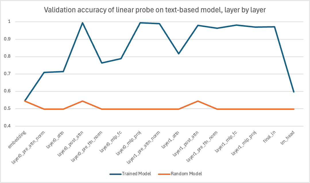
We can observe that the transformer gradually acquires a representation of the state of the Tic-Tac-Toe board, which culminates during post-attention normalization and the second layer of the MLP.

For the model trained on images, the result is very different, as the curve remains almost flat throughout the transformer.

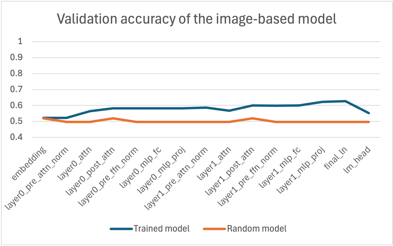
We notice that the model does not forge a representation of the Tic-Tac-Toe board, which may raise questions. To answer this, we can hypothesize that given that to solve the task (predicting the next token), one needs to have a representation to rely on at least at one point, there is no need to forge a representation when one already has the image as input, whereas it is necessary when one only has the text.

We can also look at the representation of the cells (positions), which shows some interesting symmetry and asymmetry effects.

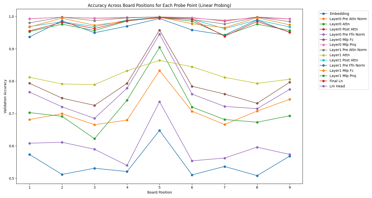
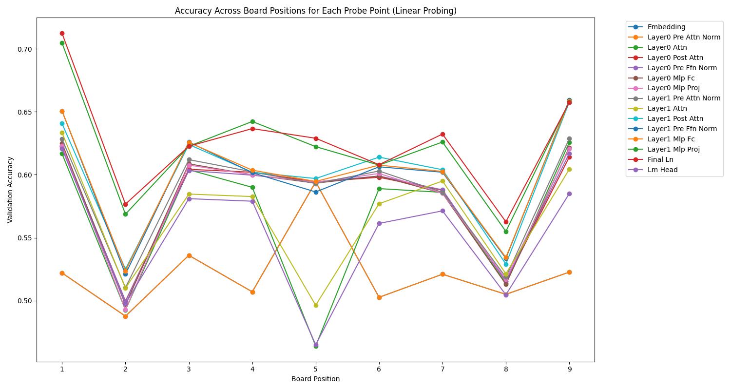
A general observation is that very often, in most layers of both models, it's the middle cell (position 5) that is best represented.

Then, we can observe beautiful symmetries, especially for the text, and certain layers, which show a geometric representation of the board that evolves depending on the layer. For example, in the image model, the pre-attention normalization layer clearly favors the central cell, while the closer we get to the output, the less this middle cell is favored, in favor of other cells, as if the analysis was performing a concentric movement towards the edges of the board.

Does the PRH hold true?

Which metrics?

Following previous literature, we define representational alignment as a measure of the similarity of similarity structures induced by two representations, i.e., a similarity metric on kernels. We give the mathematical definition of these concepts below:

• A representation is a function f : X → ℝ^n that assigns a feature vector to each input in a certain data domain X.
• A kernel, K : X × X → ℝ, characterizes how a representation measures the distance/similarity between data points. K(x_i,x_j)=⟨f(x_i),f(x_j)⟩, where ⟨·,·⟩ denotes the dot product, x_i,x_j ∈ X and K ∈ 𝒦.
• A kernel alignment metric, m : 𝒦 × 𝒦 → ℝ, measures the similarity between two kernels, i.e., how similar the distance measure induced by one representation is to that induced by another. Examples include Centered Kernel Alignment (CKA), SVCCA, and nearest neighbor metrics.

Alignment Metrics

Cycle KNN (K Nearest Neighbors Cycle)

Mathematical Definition
Let A and B be two sets of feature vectors, each of size N. For a given k:

1. Calculate the k-NN in A: For each point in A, find its k nearest neighbors in A.
2. Map these neighbors to B.
3. Calculate the k-NN in B for these mapped points.
4. Check if the original point in A is among these neighbors.

The metric is the fraction of points that "survive" this cycle.

Formula

\[ \text{Cycle\_KNN}(A, B) = \frac{1}{N} \sum_{i=1}^N \mathbb{I}(a_i \in \text{kNN}_B(\text{kNN}_A(a_i))) \]

where \(\mathbb{I}\) is the indicator function, and \(\text{kNN}_X(y)\) returns the k nearest neighbors of y in X.

Interpretation

• Range: [0, 1]
• Higher values indicate better alignment between the two feature spaces.
• A value of 1 means perfect cyclic consistency: the neighborhood structure is perfectly preserved when mapping from A to B and back.
• Lower values suggest that the local structure is not well preserved between the two spaces.

Mutual KNN (K Nearest Neighbors Mutual)

Mathematical Definition
For each point in A, check if it is among the k-nearest neighbors of its corresponding point in B, and vice versa.

Formula

\[ \text{Mutual\_KNN}(A, B) = \frac{1}{N} \sum_{i=1}^N \mathbb{I}(a_i \in \text{kNN}_B(b_i) \text{ AND } b_i \in \text{kNN}_A(a_i)) \]

where \(\mathbb{I}\) is the indicator function, and \(\text{kNN}_X(y)\) returns the k nearest neighbors of y in X.

Interpretation

• Range: [0, 1]
• Higher values indicate better mutual preservation of neighborhood between the two spaces.
• A value of 1 means that all points are mutual k-nearest neighbors in both spaces.
• Lower values suggest that the neighborhood structures in A and B are different.

CKA (Centered Kernel Alignment)

Mathematical Definition
CKA measures the similarity between two kernels after centering.

Formula

\[ \text{CKA}(K, L) = \frac{\langle K_c, L_c \rangle_F}{\|K_c\|_F \|L_c\|_F} \]

where \(K_c\) and \(L_c\) are centered kernel matrices, \(\langle \cdot,\cdot \rangle_F\) is the Frobenius inner product, and \(\|\cdot\|_F\) is the Frobenius norm.

Interpretation

• Range: [0, 1]
• Higher values indicate greater similarity between the kernel matrices.
• A value of 1 suggests that the two kernels capture identical relationships between data points.
• Lower values indicate that the kernels capture different relationships.
• CKA is invariant to orthogonal transformations and isotropic scaling.

SVCCA (Singular Vector Canonical Correlation Analysis)

Mathematical Definition

1. Perform SVD on the two feature matrices: A = U_A Σ_A V_A^T, B = U_B Σ_B V_B^T
2. Take the first d singular vectors: Ũ_A, Ũ_B
3. Perform CCA on these truncated matrices

Formula

\[ \text{SVCCA}(A, B) = \frac{1}{d} \sum_{i=1}^d \rho_i \]

where \(\rho_i\) are the canonical correlations between \(\tilde{U}_A\) and \(\tilde{U}_B\).

The steps to calculate SVCCA are:

1. Perform SVD on the two feature matrices: \[A = U_A \Sigma_A V_A^T, \quad B = U_B \Sigma_B V_B^T\]
2. Take the first d singular vectors: \(\tilde{U}_A, \tilde{U}_B\)
3. Perform CCA on these truncated matrices

Interpretation

• Range: [0, 1]
• Higher values indicate stronger correlation between the principal components of the two feature spaces.
• A value close to 1 suggests that the main directions of variation in the two spaces are strongly aligned.
• Lower values indicate that the principal components of the two spaces capture different aspects of the data.
• SVCCA is less sensitive to noise compared to simple CCA, due to the initial SVD step.

Conclusion

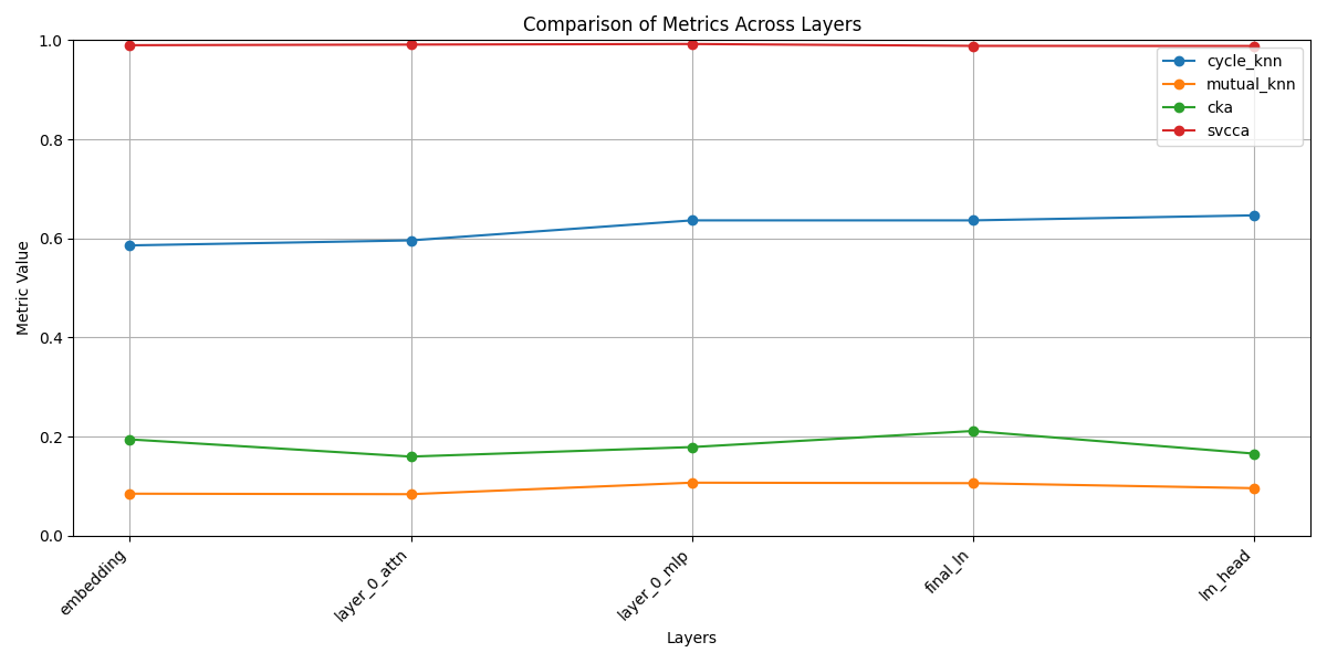
These metrics provide different perspectives on the alignment between two sets of features:

• Cycle KNN and Mutual KNN are more sensitive to local structures and can be useful for detecting fine alignments.
• CKA is more robust and captures global similarities, but may miss fine details.
• SVCCA is useful for comparing the main directions of variation, but may ignore less important features.

In practice, it is often beneficial to use several of these metrics together to get a more complete picture of the alignment between two sets of features.

The Results

Bibliography

1. Huh, M., Cheung, B., Wang, T., & Isola, P. (2024). The Platonic Representation Hypothesis. arXiv preprint.
2. Kornblith, S., Norouzi, M., Lee, H., & Hinton, G. (2019). Similarity of neural network representations revisited. In International Conference on Machine Learning (pp. 3519-3529). PMLR.
3. Raghu, M., Gilmer, J., Yosinski, J., & Sohl-Dickstein, J. (2017). SVCCA: Singular vector canonical correlation analysis for deep learning dynamics and interpretability. In Advances in Neural Information Processing Systems (pp. 6076-6085).
4. Karvonen, A. (2024). Emergent World Models and Latent Variable Estimation in Chess-Playing Language Models. arXiv preprint.